Lecture 5 - 9/14/99

Income Effects from Rand Study

• Income elasticity of demand 0.2 or less
• These estimates hold technological change constant (also true for price elasticities)
• Income elasticities from aggregate, cross-country studies over 1.0

Aggregate Cross-Country Studies (pp. 608-10, Phelps)

• Health expenditure per capita = -290 + 0.1 (per capita income)
•                                                (t=3.5)  (t=14.3)                        N=24 , elas.=1.35
• Log (per capita spending) =  -10.2  +  1.8[log(per capita income)]
•                                            (t=10.0)   (t=17.0)                         N=24 , elas.=1.8

Demand for Health Insurance

• Refer to Phelps, Chap. 10
• Health insurance is one of many insurances--third party v. first party insurance
• Demand for health insurance related to demand for health care services
• Like all other goods, demand for insurance depends on its "own" price

Concepts of Price of Insurance and Expected Loss

• Expected loss: EL=(1-p)*0 + p*L
• Expected loss=actuarial value of loss
• Example: let p=..025, L=$8,000, then EL= .975*0+.025*8,000=$200

Risk Aversion Graph

Model of Demand for Insurance:  Initial Assumptions

• A1: Individual maximizes his/her utility
• A2: Loss fixed at $* if in sick state
• A3: Probability of loss fixed
• A4: Individual chooses between two courses of action: (1) buy insurance and thereby incur small certain loss in form of insurance premium or (2) self-insure and thereby face a large loss if sick and large probability of no loss
• A5: Decreasing marginal utility of income (wealth)--same as risk aversion
• Let W3 = $10,000 (if well and self-insure); W2 = $9,800 (if insure); W1 = $2,000 (if sick and self-insure); $200 is actuarial value of loss
• At W3, U=100; at W2, U=99; at W1, U=20
• Then EU= .025*20+.975*100=98. But U =99 >EU=98

Expected Utility Graph

• Can find expected utility (EU) by drawing a straight line from end points
• A-B represents the additional amount insurance company could extract from the individual and make him as well off as self-insuring.
• The more curvature the “certainty” curve has, the more risk averse the individual is

Interpret the Cord from Expected Utility Graph

• See why cord is a straight line. Given U(W1) and U(W3) fixed, expected utility varies linearly
• Example: say p=.05, then EU=.05*20+.95*100=96; if p=.1, EU=.1*20+.9*100=92; if p=.15, EU=.15*20+.85*100=88. etc.
• If increase p, EL also up and W3-W2 up--see W2*
• If utility in the healthy state is increased, slope of cord becomes steeper and closer to the certainty curve. To see this, make U(W3)=120 (instead of 100)
• Again, if have constant MU of wealth, certainty curve and cord coincide. Then, there can be no demand for insurance

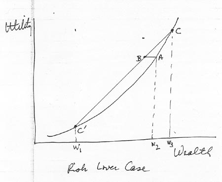
Risk Lover Graph

Risk Lover Case

• In this case, MU of wealth increases with increased wealth
• Certainty curve becomes convex to wealth (X) axis and cord on other side of curve.
• Line to cord represents amount willing to pay for opportunity to gamble
• Friedman and Savage (1948)--people have risk loving (when poor) and risk averse regions (when nonpoor)

Determinants of Demand for Insurance

• Characteristics of service.  More demand for service to be covered if (1) probability of loss in mid-range, (2) possible expenditure loss high, (3) price elasticity of demand for service is low
• Adverse selection (expected use of service)
• Loading
• Tax subsidy (varies with marginal tax rate)